Measuring population coverage bias • debiasR

Aim

This vignette shows how to measure population coverage bias in mobile-phone-derived data. The goal is simple: compare how many people are captured in the digital trace data with how many people live in each area according to a trusted benchmark.

We use the notation introduced in the previous vignette. For each Local Authority District (LAD) $i$ , let:

$U_i$ be the observed digital trace user count
$P_i$ be the benchmark population count from the 2021 Census
$c_i$ be the active-user coverage rate
$b_i$ be the coverage bias

The two core quantities are:

$c_i = \frac{U_i}{P_i}$

$b_i = 1 - c_i$

So, if an area has $c_i = 0.04$ , the digital trace data cover about 4 people per 100 residents, and the coverage bias is $b_i = 0.96$ . Lower values of $b_i$ mean better coverage. Values above zero usually mean undercoverage relative to the Census benchmark.

Load data

We use the LAD coverage table from debiasRdata. The table contains benchmark Census population counts and Locomizer-derived digital trace population counts for each LAD.

library(debiasR)
library(debiasRdata)
library(dplyr)
library(ggplot2)

coverage <- debiasRdata::coverage_lad

head(coverage)

  date                 name      code population user_count
1 2021           Hartlepool E06000001      92338       1207
2 2021        Middlesbrough E06000002     143926       1028
3 2021 Redcar and Cleveland E06000003     136531       1144
4 2021     Stockton-on-Tees E06000004     196595       1755
5 2021           Darlington E06000005     107799       1165
6 2021               Halton E06000006     128478       1744

debiasR::measure_bias() expects the benchmark population column to be called population and the digital trace population column to be called user_count. These names are already used in coverage_lad; we only rename the area code to area so the later residual diagnostic has a standard area identifier.

coverage <- coverage |>
  rename(
    area = code
  )

head(coverage)

  date                 name      area population user_count
1 2021           Hartlepool E06000001      92338       1207
2 2021        Middlesbrough E06000002     143926       1028
3 2021 Redcar and Cleveland E06000003     136531       1144
4 2021     Stockton-on-Tees E06000004     196595       1755
5 2021           Darlington E06000005     107799       1165
6 2021               Halton E06000006     128478       1744

Measure coverage bias

measure_bias() calculates the active-user coverage rate $c_i = U_i / P_i$ and the coverage bias $b_i = 1 - c_i$ .

The function returns these as:

coverage_score, which is $c_i$
coverage_bias, which is $b_i$

bias_lad <- debiasR::measure_bias(coverage)

bias_lad |>
  select(area, name, population, user_count, coverage_score, coverage_bias) |>
  head()

       area                 name population user_count coverage_score
1 E06000001           Hartlepool      92338       1207    0.013071542
2 E06000002        Middlesbrough     143926       1028    0.007142559
3 E06000003 Redcar and Cleveland     136531       1144    0.008379049
4 E06000004     Stockton-on-Tees     196595       1755    0.008926982
5 E06000005           Darlington     107799       1165    0.010807150
6 E06000006               Halton     128478       1744    0.013574308
  coverage_bias
1     0.9869285
2     0.9928574
3     0.9916210
4     0.9910730
5     0.9891928
6     0.9864257

A useful first summary is the overall coverage across all LADs. This answers: across England and Wales as a whole, what share of the Census population is captured in the digital trace population count?

bias_lad |>
  summarise(
    lad_count = n(),
    census_population = sum(population),
    digital_trace_population = sum(user_count),
    overall_coverage_score = sum(user_count) / sum(population),
    overall_coverage_bias = 1 - overall_coverage_score
  )

  lad_count census_population digital_trace_population overall_coverage_score
1       331          59597541                 654130.2             0.01097579
  overall_coverage_bias
1             0.9890242

This overall number is useful, but it can hide important local differences. A data source may have reasonable national coverage while still covering some places much better than others.

Compare LADs

The next step is to look at variation across LADs. The areas with the lowest values of $b_i$ have the strongest digital trace coverage. The areas with the highest values of $b_i$ have the weakest coverage.

bias_lad |>
  arrange(coverage_bias) |>
  select(area, name, population, user_count, coverage_score, coverage_bias) |>
  head(10)

        area             name population user_count coverage_score
1  E07000069     Castle Point      89587       1980     0.02210142
2  E07000098        Hertsmere     107827       2164     0.02006918
3  E07000066         Basildon     187571       3612     0.01925671
4  E07000113            Swale     151676       2916     0.01922519
5  E07000074           Maldon      66208       1264     0.01909135
6  E07000075         Rochford      85661       1634     0.01907519
7  E06000036 Bracknell Forest     124607       2225     0.01785614
8  E06000034         Thurrock     176001       3105     0.01764195
9  E06000035           Medway     279773       4884     0.01745701
10 E07000073           Harlow      93329       1626     0.01742224
   coverage_bias
1      0.9778986
2      0.9799308
3      0.9807433
4      0.9807748
5      0.9809087
6      0.9809248
7      0.9821439
8      0.9823581
9      0.9825430
10     0.9825778

bias_lad |>
  arrange(desc(coverage_bias)) |>
  select(area, name, population, user_count, coverage_score, coverage_bias) |>
  head(10)

        area                name population user_count coverage_score
1  E06000053     Isles of Scilly       2053          7    0.003409644
2  E09000012             Hackney     259146       1085    0.004186829
3  E09000030       Tower Hamlets     310306       1510    0.004866164
4  E07000228          Mid Sussex     152566        867    0.005682786
5  E06000016           Leicester     368571       2127    0.005770937
6  E09000019           Islington     216589       1265    0.005840555
7  E09000014            Haringey     264238       1584    0.005994596
8  E08000021 Newcastle upon Tyne     300125       1800    0.005997501
9  E07000008           Cambridge     145674        893    0.006130126
10 E07000135   Oadby and Wigston      57747        363    0.006286041
   coverage_bias
1      0.9965904
2      0.9958132
3      0.9951338
4      0.9943172
5      0.9942291
6      0.9941594
7      0.9940054
8      0.9940025
9      0.9938699
10     0.9937140

A histogram gives a quick view of how uneven coverage is across LADs.

ggplot(bias_lad, aes(x = coverage_bias)) +
  geom_histogram(bins = 30, colour = "white", fill = "#356859") +
  labs(
    x = expression("Coverage bias, " * b[i]),
    y = "Number of LADs",
    title = "Distribution of population coverage bias across LADs"
  ) +
  theme_minimal()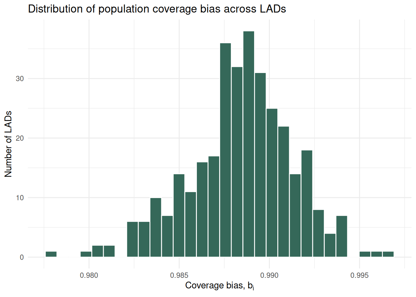

Measure distributional bias

Coverage rates tell us whether each area is over- or under-represented relative to its own benchmark population. A related question is whether the active-user population is distributed across areas in the same proportions as the Census population. For example, if an LAD contains 3% of the benchmark population, a proportionally representative active-user dataset would also place about 3% of active users in that LAD.

measure_bias_distribution() summarises this distributional comparison. It uses the benchmark population shares as the reference distribution and active user shares as the comparison distribution. Lower KL divergence and Jensen-Shannon divergence mean the active-user distribution is closer to the benchmark population distribution.

distribution_bias <- debiasR::measure_bias_distribution(
  coverage_df = coverage,
  area_col = "area",
  population_col = "population",
  user_count_col = "user_count"
)

distribution_bias$summary

# A tibble: 1 × 11
  comparison               reference_distribution comparison_distribut…¹ n_areas
  <chr>                    <chr>                  <chr>                    <int>
1 active_users_vs_populat… population             active_users               331
# ℹ abbreviated name: ¹comparison_distribution
# ℹ 7 more variables: total_population <int>, total_user_count <dbl>,
#   epsilon <dbl>, kl_population_user <dbl>, jsd_population_user <dbl>,
#   mean_abs_share_difference <dbl>, max_abs_share_difference <dbl>

The area-level output shows which LADs contribute most to the difference between the two distributions. Positive share differences mean an LAD accounts for a larger share of active users than of the benchmark population. Negative values mean the opposite.

distribution_bias$area_level |>
  dplyr::left_join(
    coverage |> dplyr::select(area, name),
    by = "area"
  ) |>
  dplyr::mutate(
    abs_share_difference = abs(share_difference_user_minus_population)
  ) |>
  dplyr::arrange(dplyr::desc(abs_share_difference)) |>
  dplyr::select(
    area,
    name,
    population_share,
    user_share,
    share_difference_user_minus_population,
    kl_contribution,
    jsd_contribution
  ) |>
  head(10)

        area          name population_share  user_share
1  E08000025    Birmingham      0.019210843 0.014197479
2  E08000032      Bradford      0.009168365 0.005338387
3  E08000003    Manchester      0.009261087 0.005936127
4  E06000016     Leicester      0.006184332 0.003251646
5  E09000030 Tower Hamlets      0.005206691 0.002308409
6  E06000035        Medway      0.004694372 0.007466403
7  E09000012       Hackney      0.004348267 0.001658691
8  E08000012     Liverpool      0.008156175 0.005738918
9  E09000025        Newham      0.005890109 0.003474843
10 E08000035         Leeds      0.013623985 0.011243939
   share_difference_user_minus_population kl_contribution jsd_contribution
1                            -0.005013364     0.005809560     1.887929e-04
2                            -0.003829978     0.004958577     2.558133e-04
3                            -0.003324960     0.004119003     1.833443e-04
4                            -0.002932686     0.003975646     2.316865e-04
5                            -0.002898282     0.004235050     2.868141e-04
6                             0.002772032    -0.002178419     1.593675e-04
7                            -0.002689576     0.004190635     3.120248e-04
8                            -0.002417257     0.002866933     1.056662e-04
9                            -0.002415266     0.003108358     1.575011e-04
10                           -0.002380046     0.002615841     5.703432e-05

Another simple check is whether coverage bias changes with area population size. This does not prove representativeness, but it helps show whether small or large areas behave differently.

ggplot(bias_lad, aes(x = population, y = coverage_bias)) +
  geom_point(alpha = 0.7, colour = "#356859") +
  geom_smooth(method = "loess", se = FALSE, colour = "#8B3A3A") +
  scale_x_log10() +
  labs(
    x = expression("Census population, " * P[i]),
    y = expression("Coverage bias, " * b[i]),
    title = "Coverage bias can vary with area population size"
  ) +
  theme_minimal()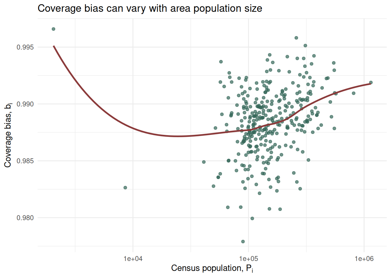

Proportional baseline

A common approach to assess whether digital trace data are a reasonable population proxy is to check whether observed user counts are proportional to benchmark population counts across areas. The logic is that areas with larger benchmark populations should also have larger observed user counts.

We refer to this as the proportional baseline because it assumes that the digital trace data capture the same share of the population in every LAD. Under this assumption, observed user counts should increase in proportion to benchmark population counts and differences in observed user counts should mainly reflect differences in population size. The comparison above showed, however, that active-user coverage rates vary across LADs. This means that a proportional relationship is useful to check, but it does not fully describe whether the data represent all areas equally.

We can use the function validate_bias_residual_structure() from debiasR to estimate this proportional baseline and inspect the residual structure, i.e. the differences between observed and expected user counts.

bias_residuals <- debiasR::validate_bias_residual_structure(
  coverage_df = coverage,
  coverage_area_col = "area",
  population_col = "population",
  user_count_col = "user_count"
)

The object returned by validate_bias_residual_structure() is a list. Each component gives different information:

summary gives the overall active-user coverage rate, the number of areas and summary measures of the residuals
residual_definitions records how the different residuals are defined and how to interpret their sign
moran_i reports spatial autocorrelation diagnostics when a neighbour table is supplied; here it is returned with missing values because we have not provided spatial neighbours
benchmark_flow_correlation reports correlations between residuals and benchmark origin or destination flow totals when a benchmark OD-flow table is supplied; here it is empty because this section only uses population counts
covariate_correlation reports the correlation between residuals and a selected area-level covariate when one is supplied; here it is returned with missing values because we have not yet added covariates
area_level contains one row per LAD with the observed count, expected count, active-user coverage rate and residuals
map_data contains the same area-level residuals, optionally joined to geometry or coordinate data when these are supplied

Some optional components may also appear if extra inputs are provided. For example, benchmark_flow_data is returned when benchmark OD flows are supplied, covariate_data is returned when a covariate is supplied and plots is returned when make_plots = TRUE.

For the rest of this vignette, we focus on three components: summary, residual_definitions and area_level.

names(bias_residuals)

[1] "summary"                    "residual_definitions"
[3] "moran_i"                    "benchmark_flow_correlation"
[5] "covariate_correlation"      "population_lm"
[7] "area_level"                 "map_data"

The summary component provides a compact description of the proportional baseline. Here, global_coverage_score is the share of the total benchmark population captured by the digital trace data across all LADs combined. This is the constant coverage rate used to calculate the expected user count in each LAD.

bias_residuals$summary

# A tibble: 1 × 14
  residual_type  selected_residual_col n_areas total_population total_user_count
  <chr>          <chr>                   <int>            <int>            <dbl>
1 coverage_score coverage_score_resid…     331         59597541          654130.
# ℹ 9 more variables: global_coverage_score <dbl>, mean_coverage_score <dbl>,
#   sd_coverage_score <dbl>, mean_selected_residual <dbl>,
#   sd_selected_residual <dbl>, moran_i <dbl>,
#   pearson_bias_benchmark_origin_flow <dbl>,
#   pearson_bias_benchmark_destination_flow <dbl>, pearson_bias_covariate <dbl>

The residual_definitions component is a useful reminder of the residuals available in the output. By default, the selected residual is coverage_score_residual.

bias_residuals$residual_definitions

# A tibble: 4 × 3
  residual                         definition                     interpretation
  <chr>                            <chr>                          <chr>
1 coverage_score_residual          coverage_score - global_cover… Positive valu…
2 user_count_residual              user_count - expected_user_co… Positive valu…
3 standardized_user_count_residual user_count_residual / sqrt(ex… Positive valu…
4 population_lm_residual           user_count - fitted(user_coun… Positive valu…

The area_level component is the main table used for interpretation. It keeps the original population and user counts, adds the expected user count under the proportional baseline and then calculates residuals for each LAD.

bias_residuals$area_level |>
  select(
    area,
    population,
    user_count,
    expected_user_count,
    coverage_score,
    coverage_score_residual,
    selected_residual
  ) |>
  head()

       area population user_count expected_user_count coverage_score
1 E06000001      92338       1207            1013.483    0.013071542
2 E06000002     143926       1028            1579.702    0.007142559
3 E06000003     136531       1144            1498.536    0.008379049
4 E06000004     196595       1755            2157.786    0.008926982
5 E06000005     107799       1165            1183.179    0.010807150
6 E06000006     128478       1744            1410.148    0.013574308
  coverage_score_residual selected_residual
1            0.0020957494      0.0020957494
2           -0.0038332327     -0.0038332327
3           -0.0025967426     -0.0025967426
4           -0.0020488102     -0.0020488102
5           -0.0001686417     -0.0001686417
6            0.0025985164      0.0025985164

The default residual, coverage_score_residual, is local coverage minus overall coverage:

$c_i - \bar{c}$

Here, $\bar{c}$ is the overall active-user coverage rate. Positive values mean the LAD is covered more than expected under the proportional baseline. Negative values mean the LAD is covered less than expected.

Because the vignette focuses on bias, we also create a bias residual:

$r_i = b_i - \bar{b}$

where $\bar{b} = 1 - \bar{c}$ . Positive values of $r_i$ mean the LAD has more coverage bias than expected under the proportional baseline. Negative values mean it has less coverage bias than expected.

residual_lad <- bias_residuals$area_level |>
  mutate(
    baseline_coverage_score = global_coverage_score,
    baseline_coverage_bias = 1 - global_coverage_score,
    residual_bias = coverage_bias - baseline_coverage_bias
  ) |>
  left_join(
    coverage |> select(area, name),
    by = "area"
  )

residual_lad |>
  select(
    area,
    name,
    population,
    user_count,
    baseline_coverage_score,
    coverage_score,
    coverage_bias,
    residual_bias
  ) |>
  head()

       area                 name population user_count baseline_coverage_score
1 E06000001           Hartlepool      92338       1207              0.01097579
2 E06000002        Middlesbrough     143926       1028              0.01097579
3 E06000003 Redcar and Cleveland     136531       1144              0.01097579
4 E06000004     Stockton-on-Tees     196595       1755              0.01097579
5 E06000005           Darlington     107799       1165              0.01097579
6 E06000006               Halton     128478       1744              0.01097579
  coverage_score coverage_bias residual_bias
1    0.013071542     0.9869285 -0.0020957494
2    0.007142559     0.9928574  0.0038332327
3    0.008379049     0.9916210  0.0025967426
4    0.008926982     0.9910730  0.0020488102
5    0.010807150     0.9891928  0.0001686417
6    0.013574308     0.9864257 -0.0025985164

The largest positive residuals are LADs where digital trace coverage is lower than expected from the national baseline.

residual_lad |>
  arrange(desc(residual_bias)) |>
  select(area, name, population, user_count, coverage_score, coverage_bias, residual_bias) |>
  head(10)

        area                name population user_count coverage_score
1  E06000053     Isles of Scilly       2053          7    0.003409644
2  E09000012             Hackney     259146       1085    0.004186829
3  E09000030       Tower Hamlets     310306       1510    0.004866164
4  E07000228          Mid Sussex     152566        867    0.005682786
5  E06000016           Leicester     368571       2127    0.005770937
6  E09000019           Islington     216589       1265    0.005840555
7  E09000014            Haringey     264238       1584    0.005994596
8  E08000021 Newcastle upon Tyne     300125       1800    0.005997501
9  E07000008           Cambridge     145674        893    0.006130126
10 E07000135   Oadby and Wigston      57747        363    0.006286041
   coverage_bias residual_bias
1      0.9965904   0.007566148
2      0.9958132   0.006788963
3      0.9951338   0.006109628
4      0.9943172   0.005293006
5      0.9942291   0.005204855
6      0.9941594   0.005135237
7      0.9940054   0.004981196
8      0.9940025   0.004978291
9      0.9938699   0.004845666
10     0.9937140   0.004689751

The most negative residuals are LADs where coverage is higher than expected.

residual_lad |>
  arrange(residual_bias) |>
  select(area, name, population, user_count, coverage_score, coverage_bias, residual_bias) |>
  head(10)

        area             name population user_count coverage_score
1  E07000069     Castle Point      89587       1980     0.02210142
2  E07000098        Hertsmere     107827       2164     0.02006918
3  E07000066         Basildon     187571       3612     0.01925671
4  E07000113            Swale     151676       2916     0.01922519
5  E07000074           Maldon      66208       1264     0.01909135
6  E07000075         Rochford      85661       1634     0.01907519
7  E06000036 Bracknell Forest     124607       2225     0.01785614
8  E06000034         Thurrock     176001       3105     0.01764195
9  E06000035           Medway     279773       4884     0.01745701
10 E07000073           Harlow      93329       1626     0.01742224
   coverage_bias residual_bias
1      0.9778986  -0.011125629
2      0.9799308  -0.009093393
3      0.9807433  -0.008280916
4      0.9807748  -0.008249398
5      0.9809087  -0.008115556
6      0.9809248  -0.008099400
7      0.9821439  -0.006880348
8      0.9823581  -0.006666153
9      0.9825430  -0.006481218
10     0.9825778  -0.006446445

ggplot(residual_lad, aes(x = residual_bias)) +
  geom_vline(xintercept = 0, colour = "grey40") +
  geom_histogram(bins = 30, colour = "white", fill = "#6B5B95") +
  labs(
    x = expression("Bias residual relative to proportional baseline, " * r[i]),
    y = "Number of LADs",
    title = "Some LADs depart from the constant-coverage baseline"
  ) +
  theme_minimal()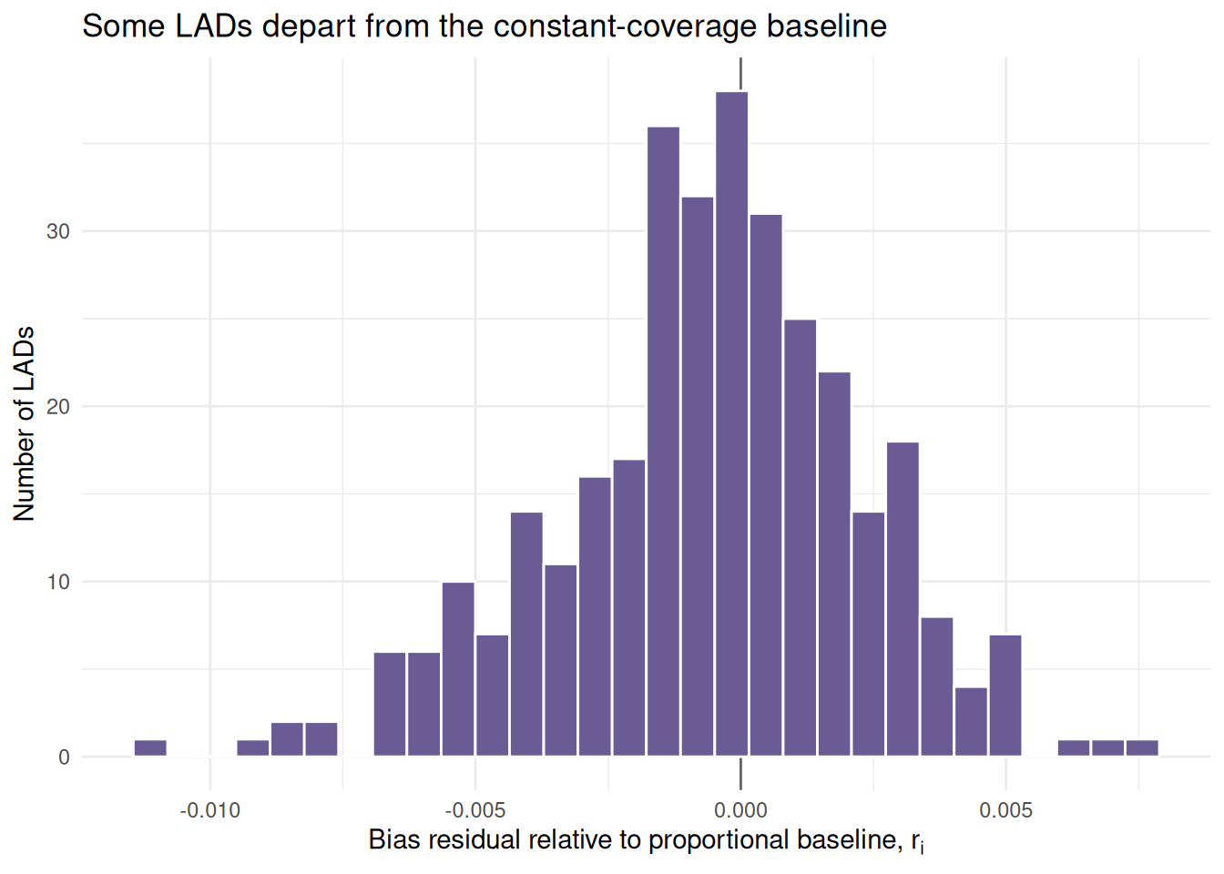

Interpretation

We have seen that population coverage bias tells us how much of the benchmark population is visible in the digital trace data. But, is this coverage roughly constant across places, or are some LADs more visible in the data than others?

In practice, we find that coverage tends to be uneven. Some LADs are overcovered or undercovered relative to the national average coverage rate. These departures raise a representativeness question: why is a particular place more or less visible than expected? One possibility is that the area contains a larger share of population groups (e.g. people aged 20-29) that are more or less likely to appear in the digital trace data.

The key message is that high overall coverage is not the same as representativeness. A data source can capture many people in total while still representing some places and population groups better than others. So, our next step is to ask whether residual coverage bias is associated with area characteristics such as age structure, socioeconomic composition or rurality.